In statistics, not all data follows the familiar bell-shaped curve of the normal distribution. Some real-world data are positively skewed, meaning values cluster near the lower end but stretch toward higher values. The Lognormal Distribution is one such model used to describe this kind of data. It is especially important in fields like finance, engineering, and reliability analysis, where data cannot go below zero but can grow to large positive numbers.
What Is the Lognormal Distribution?
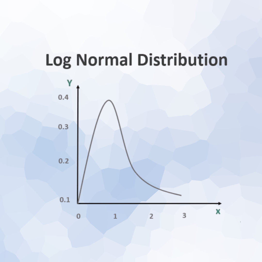
The Lognormal Distribution is a type of continuous probability distribution where the logarithm of the variable follows a normal distribution. In simpler terms, if you take the log of the data values, the result would form a normal (bell-shaped) curve.
Unlike the normal distribution, which is symmetric, the lognormal distribution is right-skewed — meaning it has a long tail toward higher values. This makes it useful for modeling data that cannot be negative and where large values occasionally occur.
Why the Lognormal Distribution Is Important
Many natural and economic processes grow multiplicatively, not additively. For instance, product lifetimes, income levels, or stock prices can multiply over time rather than increase by fixed amounts. The lognormal distribution captures these multiplicative effects accurately.
Key characteristics:
- Data values are always positive.
- Most values are near the lower range, but a few can be much higher.
- It effectively represents growth-based or time-dependent phenomena.
This makes the lognormal distribution an essential tool in reliability analysis, risk modeling, and environmental studies.
Real-Life Example: Product Lifetimes in Manufacturing
Consider an electronics manufacturer studying the lifespan of light bulbs. Most bulbs last around 1,000 hours, but a few exceptional ones last much longer — 2,000 or even 3,000 hours. The data distribution is not symmetric; it has a long right tail representing those few long-lasting bulbs.
The lognormal distribution fits this pattern perfectly because:
- The data cannot go below zero (a bulb can’t have a negative lifespan).
- Lifespans vary greatly, with many short and a few very long durations.
- The variation increases multiplicatively due to material or production differences.
Engineers use the lognormal distribution to estimate product reliability, predict warranty claims, and optimize maintenance schedules.
Applications Across Industries
The lognormal distribution is widely used in various fields:
- Finance: To model stock prices and investment returns, which grow over time.
- Engineering: For failure time analysis and product reliability.
- Environmental science: To describe particle sizes, pollution levels, or rainfall amounts.
- Economics: For modeling income distribution, where most people earn moderate incomes while a few earn very high ones.
Conclusion
The Lognormal Distribution is a powerful tool for analyzing positively skewed data that grows or changes multiplicatively over time. Unlike the symmetric normal distribution, it captures the reality of unequal or unpredictable growth found in manufacturing, finance, and natural phenomena. By understanding and applying the lognormal model, analysts and engineers can make more accurate predictions, improve product designs, and better assess risk in complex systems.